Population and Samples
Lecture 3

Population and Samples

1. Populations and samples

   1. Depends on data or survey

   2. Example

      1. Population – survey CEOs of the world’s top 500 corporations

      2. Parameters

         1. Mean, m

         2. Standard deviation, s

      3. Sample – population has too many individuals

      4. Choose sample of population

   3. Conditions

      1. Every individual in a population has a known non-zero chance of being sampled

      2. Equal chance for everyone

      3. Has to be independent ; choosing one does not influence the choice for choosing another

         • Then we have a random sample

   4. Have to be careful when defining a population

      1. Book – each member of population has a number

      2. Use a random number table to randomly select individuals

      3. Excel – the function is =rand( )

         1. Distributed uniform (0, 1)

         2. X ~UNIF(0, 1)

      4. Select numbers between 0 and 1,000

         1. =round(1000*rand(), 0)

         2. The round function rounds a number to the integer

      5. Each time you change something in Excel, Excel recalculates the random numbers

         1. Use Copy and Past Special to freeze the random numbers and stop them from changing

2. Trick – Generate random numbers with any distribution

   1. Example – generate normally distributed random numbers

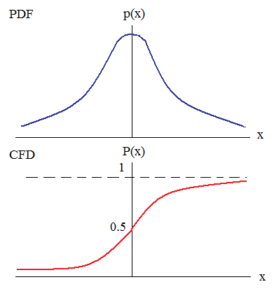
      1. Probability Density Function (PDF) – a function that associates each value of a discrete random variable with the probability that this value will occur.

         1. Denoted as p(x) or f(x)

      2. Cumulative Density Function (CDF) – integral of a probability function

         1. Denoted by a capital letter, such as P(x) or F(x).

          If you sum over all probabilities, then it has to equal one

3. A PDF and CDF is shown below

2. Use UNIF to get probability between 0 and 1

   1. Find the inverse for P(X) using that random number

   2. To randomly create a normally distributed variable with mean and standard deviation, then the Excel function is

   3. =norminv(rand(), mean, standard deviation)

3. Example

   1. Find the random numbers for the distribution, X _i~N(10, 25)

      1. The notation is X _i~N( m, s ²)

      2. The Excel function is = norminv(rand(), 10, 5)

   2. Can use this method to find random numbers from any distribution

3. Stratified Random Sampling

   1. You take a sample and then you divide a sample by gender (male or female)

   2. Then you divide by age, creating the four categories

      1. 0 – 30 years

      2. 31 – 40 years

      3. 40 – 60 years

      4. > 60 years

   3. You have a total of eight compartments

      1. You randomly select individuals and fill the compartments equally

      2. Each compartment has 10 individuals

   4. Unfortunately, males/females and age categories may not be distributed evenly

      • Forcing the compartments may create a biased sample

4. Unbiasedness – on average, the mean of a sample will equal its true parameter value

   1. The notation is E( ) = m

   2. E stands for expected value

   3. Precise – the study is repeatable, if we took another sample, we get similar results

   4. Nonrandom samples – makes our parameter estimates biased

      1. Some people in the population will never be selected; they may be transient

      2. Some people may not fill out the surveys

      3. Some people may lie on surveys

5. Block Randomization

   1. Use Table F and choose block size 2, 4, 6, 8, and 10

   2. Example – testing effectiveness of a new drug

      1. We have 8 patients, and choose block size 8

      2. Four patients get the new drug, while four patients get the placebo

      3. Our study has 8 patients who have a unique number between 1 and 8

      4. Patients could be a biased sample; however, we are testing drug’s effectiveness

      5. Then we have 8 patients who get the following treatments

6. Standard Error

   1. Each time we take a sample, we get a different mean

   2. Example

      • Sample 1: =29.3

      • Sample 2: =33.3

• Sample 100: =27.7

3. We do not want to keep taking samples to find the variability in the mean

4. The standard error (SE) gives the variability in the mean for repeated sampling

5. The formula

6. As the sample size increases, the standard error decreases

7. With an infinite sample size, we know the true parameter for the mean

7. Binominal Distribution

   1. We have two states,

      1. P is probability that Event A happens

      2. 1 – P is probability that Event A does not happen

   2. The states or events are mutually exclusive

      1. We sampled 80 people and 43 went to college

      2. The mean for people going to college (the event)

         1. P = 43 / 80 = 0.5375

      3. The probability for people who did not go to college

         1. 1 – P = (80 – 43) / 80 =1 – 0.5375 = 0.4625

   3. The variance

      • var(P) = P(1 – P) = 0.5375(0.4625) = 0.249

   4. The standard error is

      • 

   5. It is possible to keep probability of events in percents.

      • The mean and SE are the same