Correlation and Regression
Lecture 10

Correlation

Correlation – measure of linear association between two variables

1. Pearson’s correlation

   1. Key word is “linear”

2. cov shows how two variables vary together

3. If X = Y, then

4. var(X) is population variance

5. If we estimate cov(X, Y), var(X), and var(Y) by population formulas, then

2. Correlation ranges [-1, +1]

   1. If r = -1, then

2. If r = +1, then

3. If r = 0, then

4. Note – exponential function would have a high correlation, but it is not linear

3. First step

   1. Construct a scatter diagram of the data

   2. What does the data look like?

4. Define

   1. X is the independent variable

   2. Y is the dependent variable

   3. Define the function, Y = f(X)

      1. Y is a function of X

      2. Establishes causality

      3. Correlation does not establish causality

5. Example – Chest pains and shortness of breath may have a high positive correlation

   1. One does not cause the other

   2. Clogged arteries can cause these two symptoms

   3. Be very careful, correlation does not establish causality

6. Correlation t-statistic

   1. Assumptions

      1. Both variables are normally distributed

      2. Both have a linear relationship

   2. Hypothesis test

3. The t-test is:

4. Notation

   1. r is the correlation coefficient

   2. n is the number of observations

   3. df = n – 2

   4. The 2 is because correlation involves two variables

7. Spearman Rank Correlation

   1. Reduces problems with outliers

   2. Can handle non-linear relationships, like exponential functions

Regression Equation

1. You are imposing a relationship onto the variables

1. Y_i is the dependent variable

   1. Value is obtained from X_i and u_i

2. X_i is the independent variable

3. b₁ and b₂ are parameters

   1. These are estimated from the data

4. u_i is the random noise term, u_i ~ N(0, s²)

   1. Notation

      1. N is normally distributed

      2. Mean is 0

      3. Variance is s²

   2. Having normally distributed noise allows us to calculate confidence intervals and perform hypothesis testing

   3. Estimates of b₁ and b₂ and predictions of Y_i are influenced by the variance of the noise

2. We find the and that minimizes the errors for the data points

   1. Some errors are positive

   2. Other errors are negative

   3. We cannot add the errors because they may cancel

   4. We square the errors terms to make them all positive

3. Derivation

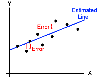
Starting with the equation

Solve for u_i, which yields

Square the errors to make them positive

This is only for one data point. We want to minimize the total errors of all the data points.
     Sum over all the data points
     Define Sum of Squared Errors (SSE)

We want to find the minimum, thus we take the first partial derivatives with respect to the betas

The second step is the Chain Rule from Calculus.  I can put the 2 in front of the summation because each term in the summation has a 2.  Set the partial derivative to zero, in order to find minimum value

Now solve equation for b₁,   It is debatable when you should add hats to the estimators.  I added at this step when partial was set to zero

Summation is a linear operator.  We can apply the summation to all terms in parenthesis
     b₁ is constant that is summed n times
     b₂ is constant and multiplied by all X’s in summation
     Can bring this to the front

The last step works because we substitute the average for y and average for x into the equation.  Repeating these steps to get the estimator for b₂

Similarly, set the partial to zero and solve for b₂,

We substitute the estimator for b₁ into the equation, , which yields

I did not break the last summation apart.  This is to solve for the estimator for b₂

4. This is only good for one X variable. We can generalize least squares to Multiple Regression. There is k parameters to estimate.

5. Example – Demand for Pepsi

   1. Q is quantity and P is market price

2. Use least squares to find betas

3. I fitted a line through my data points that gives me the best fit

Goodness of Fit

1. The goodness-of-fit measure is, R².

1. If R² = 0, then the regression equation has no fit
2. If R² = 1, then a regression equation has a perfect linear fit
3. Also, n = k which is algebraic system
4. Problem – As the number of x variables increases, R² always gets larger

2. Adjusted R² - Penalize the goodness of fit if more variables are added

.

1. As the number of independent variables increase, the penalty increases, but the error could decrease if new variables explain ‘y’ better.
2. Sometimes can be negative, indicating a very poor fit
3. Note – Very important; it has to be the same y variable
4. One model it cannot be y and in another it is ln (y)

Analysis of Variance )ANOVA)

In terms of regressions, ANOVA is used to test hypothesis in many types of statistical analysis
Sum of Squared Total (SST) is defined as:

.

Y_i is the dependent variable in the regression.  The is the total variation for observation i.
Sum of Squared Regression (SSR) is defined as:

.

This is the variation explained by the regression
Sum of Squared Errors (SSE), which was earlier defined as:

SSE is the amount of variation not explained by the regression equation.  Thus, SST = SSR + SSE, which is proved in the lecture.
We can use this information to calculate the R² statistic, showing the relationship:

Problem – the more parameters added to the regression, the higher the R².

R² = 1, if n = k, the number of parameters equal observations

Now we need the degrees of freedom for each measure:

          Sum of Squared Regression (SSR)      df =k – 1

          Sum of Squared Errors (SSE)             df = n – k

          Sum of Squared Total (SST)               df = n – 1

We calculate the Mean Square (MS)

         Regression (MS) = SSR / (k – 1)

          Residual (MS) =SSE / (n – k)

          Total (MS) NA

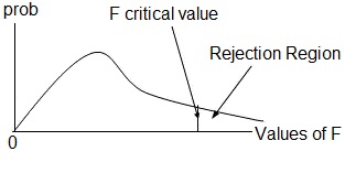
• Additional information

  • When you have a variable with a normal distribution

    • If you add or subtract if from other variables with a normal distribution, then it is still normally distributed

    • Calculating a mean is a first moment

  • If you square a random variable with a normal distribution, then you get a chi-square distribution with degrees of freedom.

    • The squares are variances and called the second moment

    • All the Mean Squares are distributed as chi squares

• AF-distribution – can test a whole group of hypothesis or test a whole regression model

  • F- test can test many other things

  • The F-test is a ratio of two chi-squares

  • The F-test is a one-tailed test associated with the right-hand tail.

  • Squaring makes all terms positive

• The F-distribution and test is as follows:

The hypothesis test

     H₀: Regression model does not explain the data, i.e. all the parameters estimates are zero

     H_a: Regression model does explain the model, i.e. at least one parameter estimate is not zero

First, we need the critical value: a = 0.05, df₁ = 1, and df₂ =58

     In Excel, =finv(0.05,1,58)

     F_c = 4.00

Excel calculates the ANOVA

Calculate the F-value =

The computed F exceeds the F_c, so reject the H₀, and conclude at least one parameter is not equal to zero.
     How many observations? 10
     How many parameters, k? 4

     Degrees of freedom for error df = 10 – 4 = 6
     Degrees of freedom for total df = 10 – 1 = 9

Trend Regression

1. Time series – date collected over time

   1. Could have patterns over time

2. Trend variables always start at 1

3. You never put in the year

4. You can add powers of the trend

2. An example

1. Use adjusted R² to find stopping point

2. Choose the Regression with largest adjusted R²

3. Note – R² will always take the largest regression

3. Exponential Regression

1. Transform equation until linear in parameters by taking the natural logarithm of both sides

2. Re-parameterize to avoid the natural log in the intercept

3. Just take the natural logarithm of the variables except the trend variable and then do a standard linear regression